CourseKata Chapter 9 (9 to 11)
Linear Regression
Mansour Abdoli, PhD
Overview / Goals
- Correlation (r)
- Correlation matrices
- Relationship between r and R²
- Null distribution of slopes
- Limits of regression models
Two Numerical Variables
Previously we modeled:
- response variable (y)
- explanatory variable (x)
with regression
\[ \hat{y} = b_0 + b_1x \]
Key question:
How strong is the relationship?
Pearson’s Correlation (r)
Pearson’s (r):
- measures strength and direction
- of a linear relationship
- between two quantitative variables
Range:
\[ -1 \le r \le 1 \]
Interpreting r
| r value | Meaning |
|---|---|
| close to 1 | strong positive relationship |
| close to -1 | strong negative relationship |
| close to 0 | weak or no linear relationship |
Important:
Correlation measures linear association.
Example Scatterplot
Questions:
- What direction is the relationship?
- How strong is the relationship?
Calculating Correlation
Pearson’s r (using R):
Interpretation:
- sign → direction
- magnitude → strength
Correlation Matrix
Pairwise correlations for multiple variables:
Example:
       mpg    wt    hp  disp
mpg   1.00 -0.87 -0.78 -0.85
wt   -0.87  1.00  0.66  0.89
hp   -0.78  0.66  1.00  0.79
disp -0.85 0.89 0.79 1.00- Practice: Interpret some the values.
Relationship Between r and R²
Understanding the Slope
Recall the regression model: \[\hat{y} = b_0 + b_1x\]
The slope (b_1):
change in predicted (y) for a one-unit increase in (x).
But how do we know if this slope is meaningful?
Null Model Idea
The slope is zero: \(\beta_1=0\)
No relationship between \(x\) and \(y\)
Any observed relation is due to random variation.
- Simulate random variation:
- Shuffle the response variable.
- Recalculate the slope.
- Repeat many times.
Simulation Example
Limitation of Regression
- Association vs causation
- Extrapolation
- Linearity assumption
Association vs Causation
Regression detects association, not causation.
Example:
Ice cream sales ↑
Drowning incidents ↑
- Does ice cream cause drowning?
Extrapolation
Where models are reliable?
- within the observed data range.
Example:
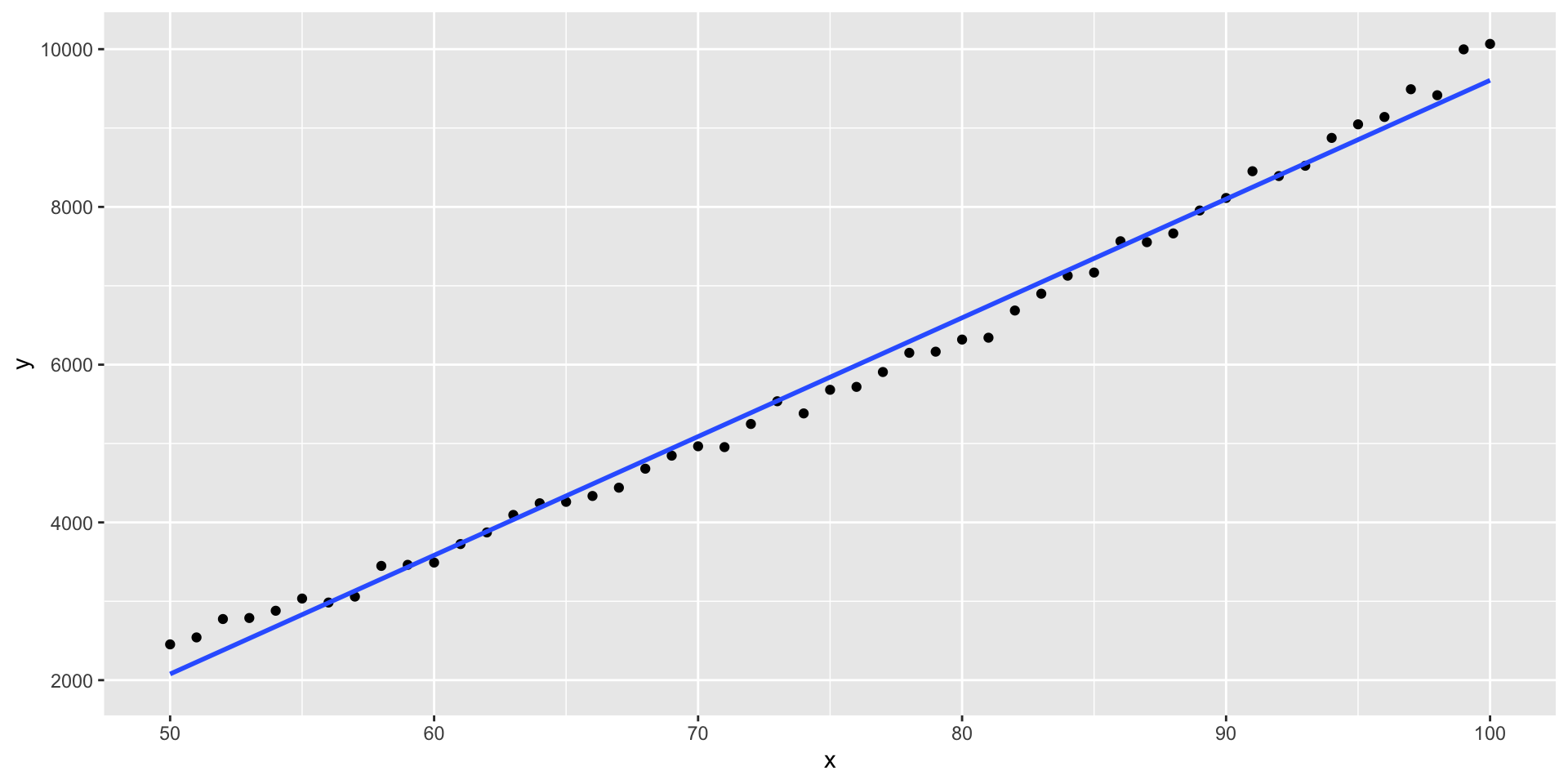
Linearity Assumption
Linear regression assumes:
\[\text{relationship = straight line}\]
But some relationships are curved.
Example patterns:
- quadratic
- exponential
- saturation effects
Example Nonlinear Pattern
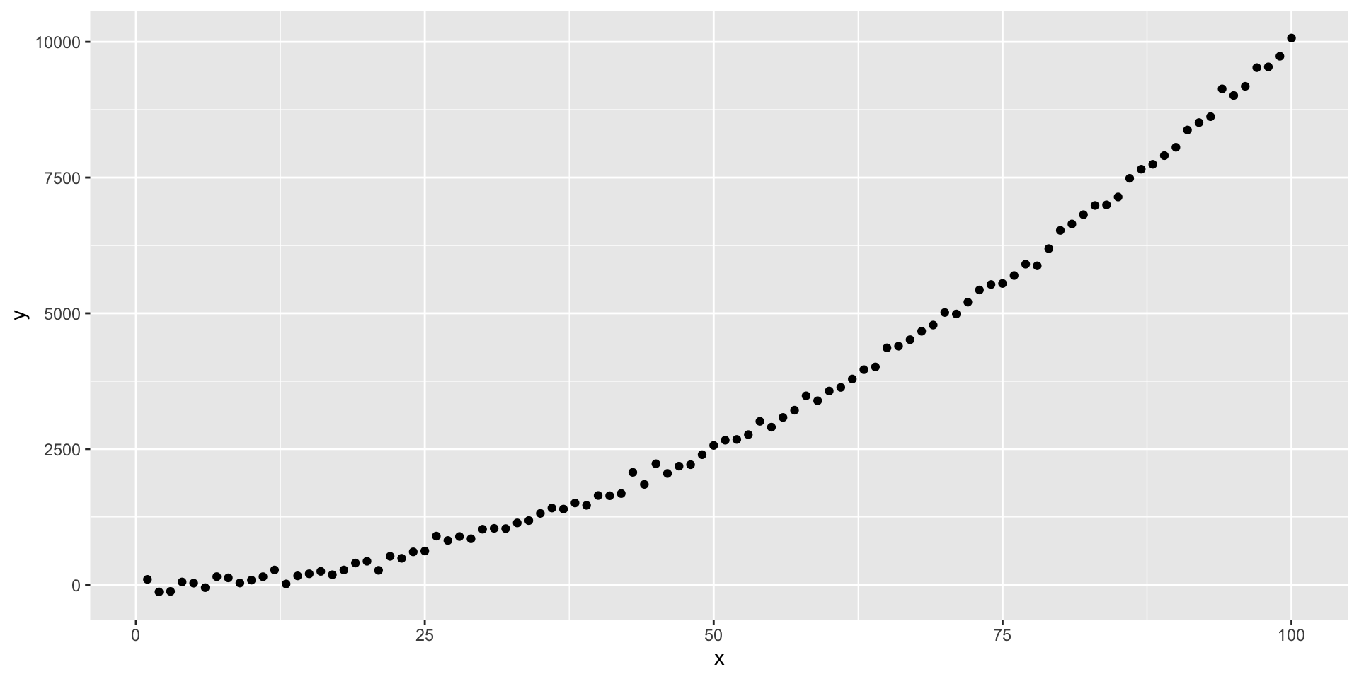
A straight line would not describe this well.
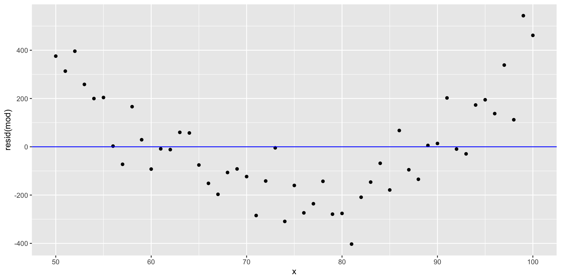
Diagnosing Linearity
We check:
- scatterplots
- Linear relation
- residual plots
- No systematic pattern.
Key Takeaways
- Correlation (r): measures strength of linear association
- Relationship: \(R^2 = r^2\)
- Null slope distribution:
- helps evaluate whether slopes occur by chance
- Regression limitations:
- association ≠ causation
- avoid extrapolation
- check linearity
CourseKata Ch. 9