CourseKata Chapter 3.10–3.13
The DGP • Sampling Variation • Simulations
Session goals
By the end of today, you can:
- Explain what Data Generating Process (DGP) means.
- Use bottom‑up vs top‑down thinking to connect data ↔︎ DGP
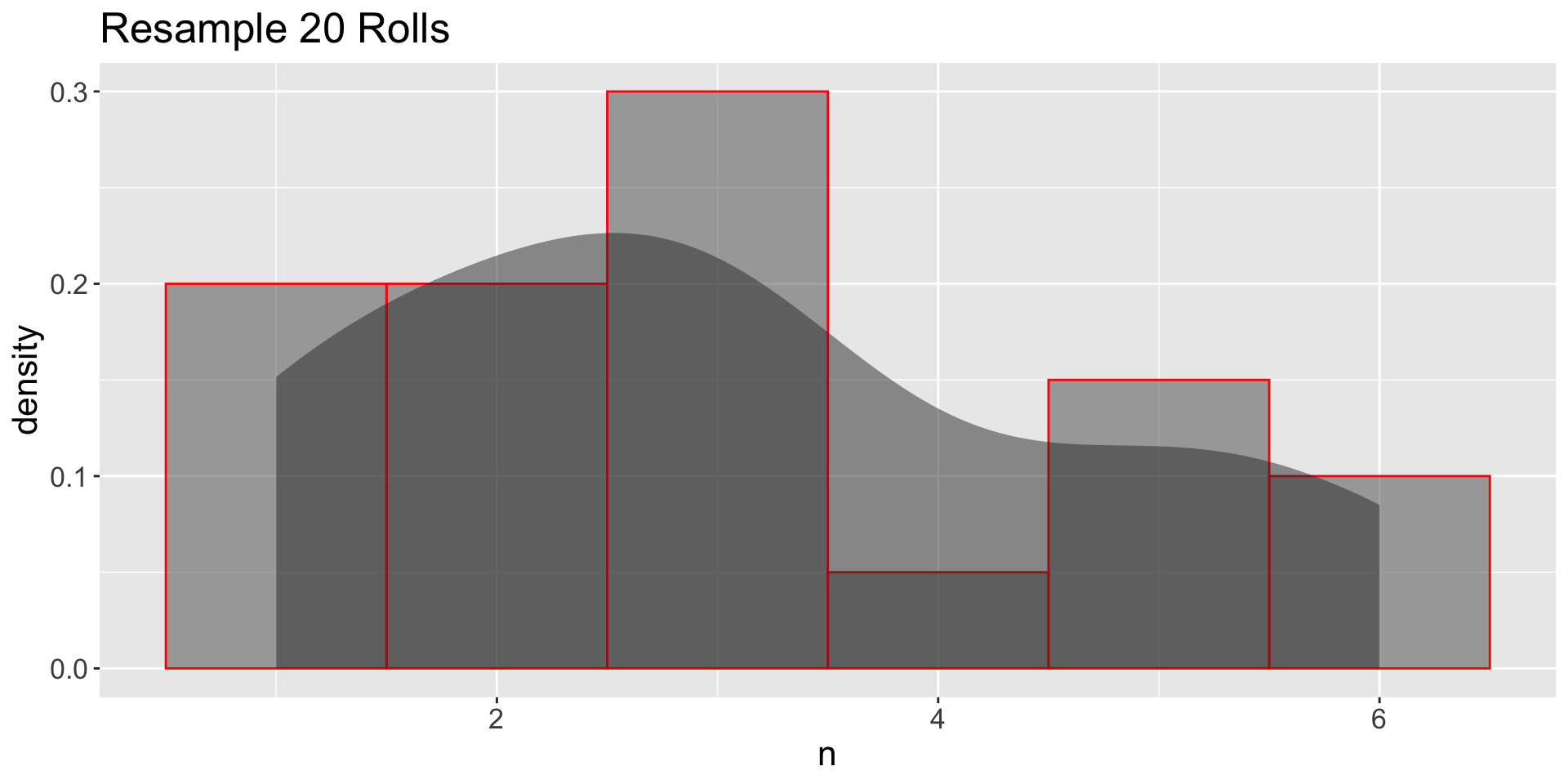
- Simulate a DGP with
sample() / resample() and visualize results
- Explain sampling variation and why small samples can look “weird”
- Use simulations to see the law of large numbers in action
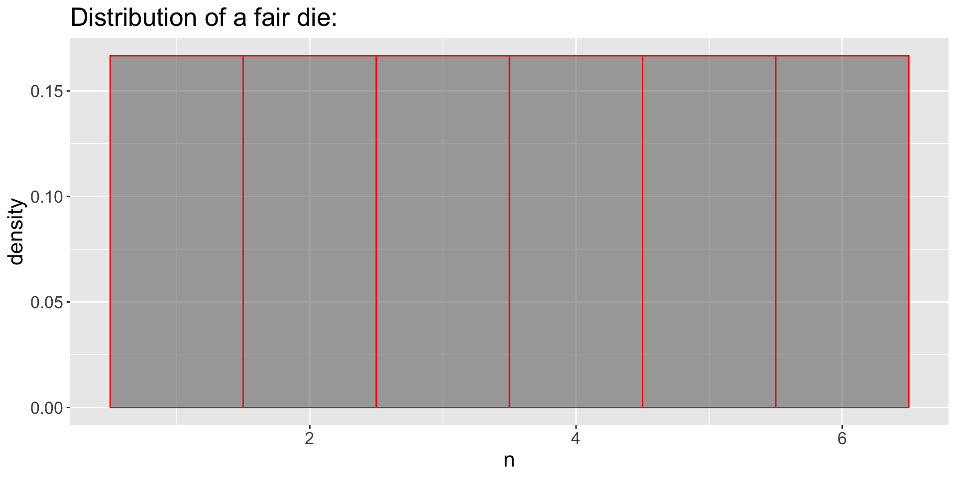
3.10 The Data Generating Process (DGP)
Data Generating Proccess (DGP)
- Distributions Represents Variability in Data
- Variation in part depends on the DGP
- Key Idea: “What DGP generated population variability?”
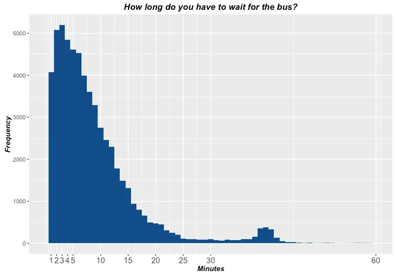
Quick example: bus wait times (source)
- DGP thinking =
using context to explain the distribution:
- schedules?
- passenger behavior?
- delays, traffic, bunching?
3.11 Back-and-forth: data ↔︎ DGP
Two moves statisticians make
- Top‑down: Theory of DGP → Expected Distribution
- Bottom‑up: Observed Distribution → Predict Population/DGP
Sampling and Resampling
- Pair prompt:
- Why do we get different numbers?
- What stays the same?
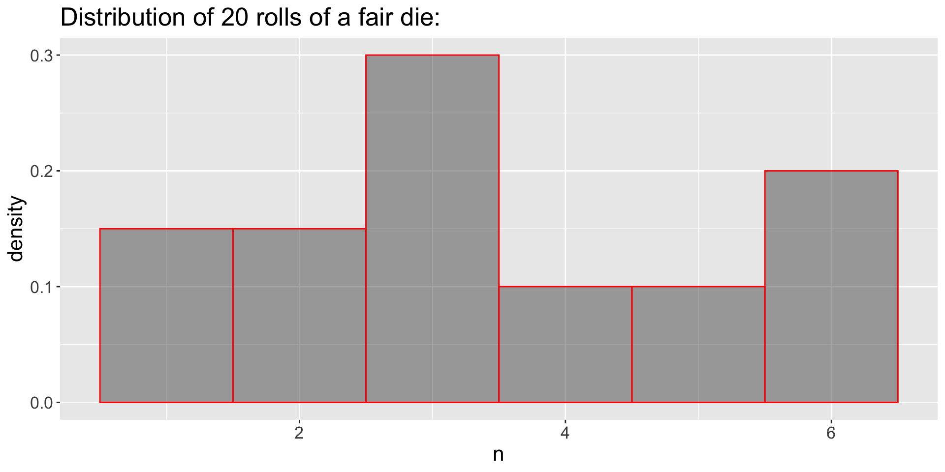
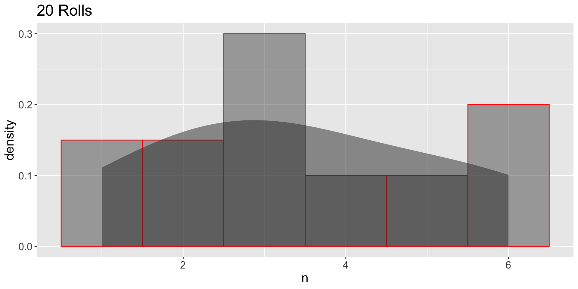
3.12 From DGP → population → samples
GDP: Independent Samples
- Sample with replacement (Independet Samples)
- What happens if
replace = FALSE (default)?
- How the distribution resembles the population?
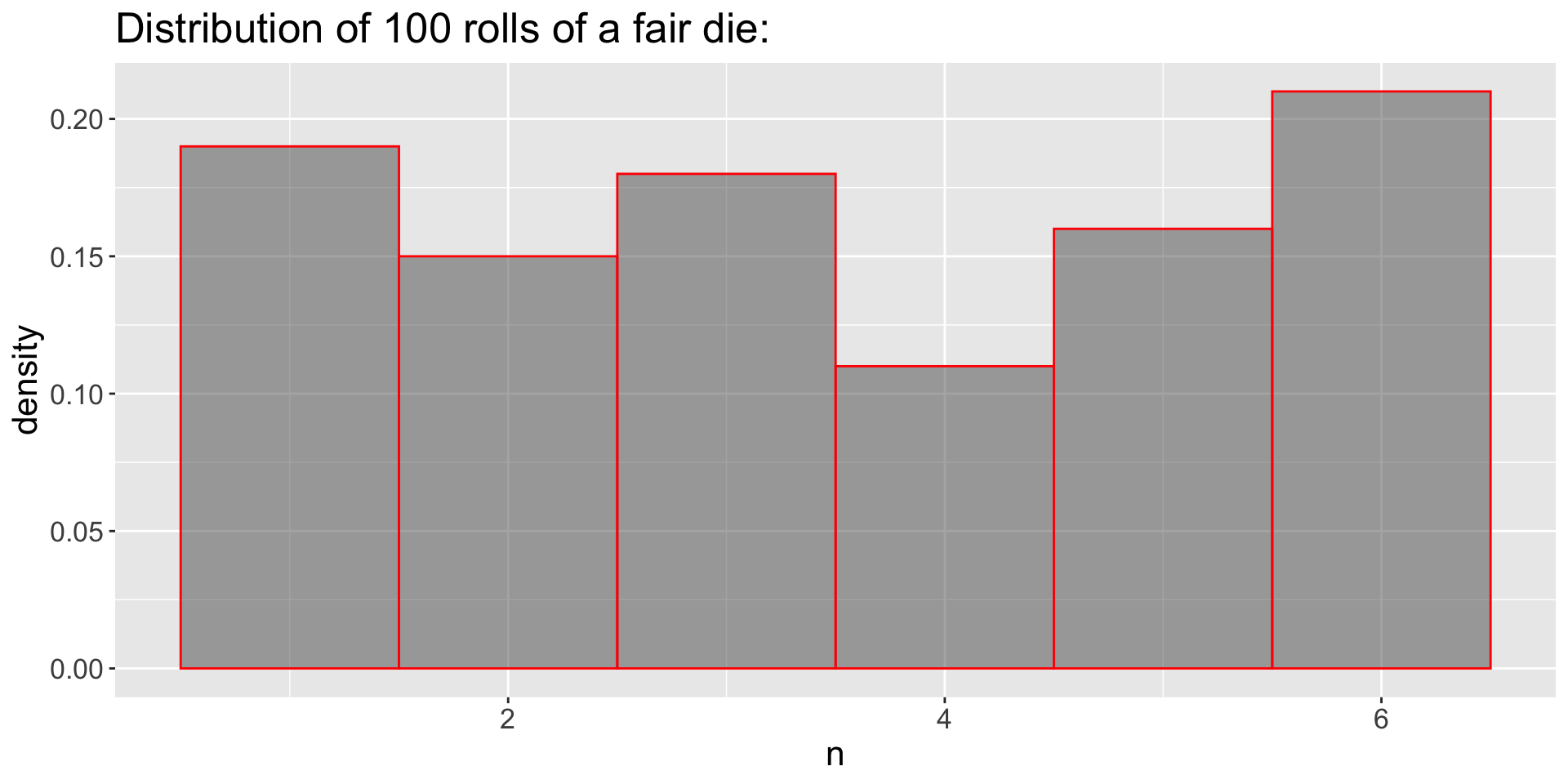
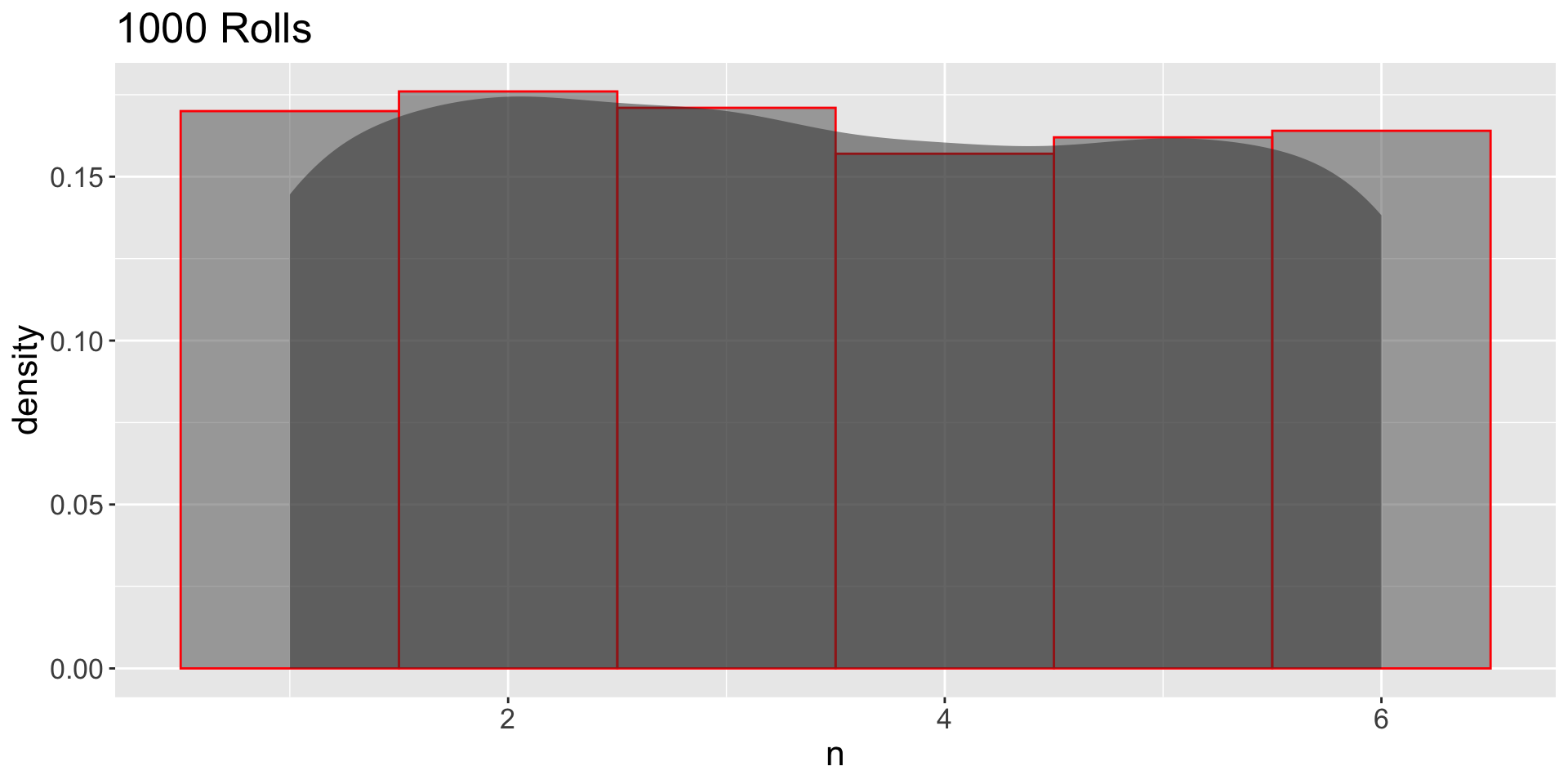
GDP: Large Independent Samples
- 1000 independent samples:
- Which one (10 or 1000) looks more like the population?
- Which one has more sampling variation?
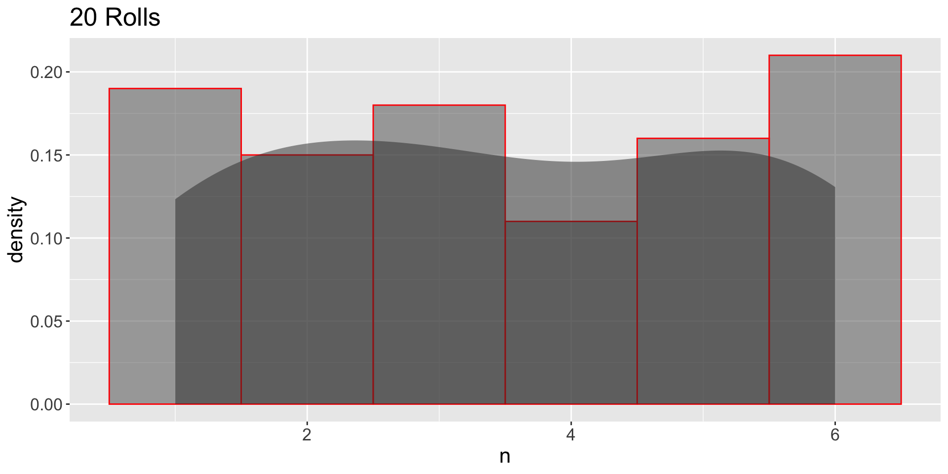
3.13 Weird DGPs and their samples
Weird populations can exist
Sampling from the Weird Population
- Which sample “reveals” the W-shape better?
- Which DGP is more variable?
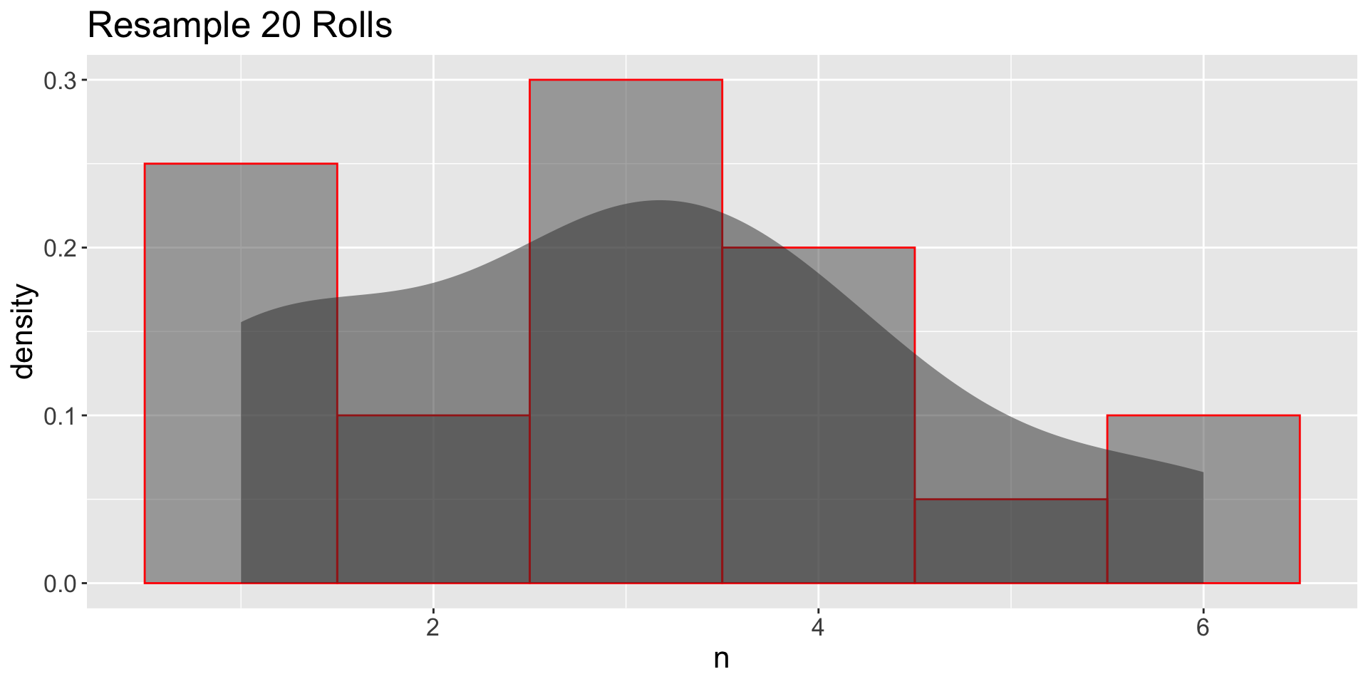
Law of Large Numbers
- As sample size increases:
- the sample distribution tends to resemble the population distribution more closely.
- A single small sample could do the same but less likely to do so:
- Small samples can be misleading.
- Law of Large Numbers works better on Statistics than Distribution! Why?