CourseKata Chapter 11
Model Significance (2)
Mansour Abdoli, PhD
Overview / Goals
- Complex v. Simple Models
- Type I Error Inflation
- Single Model Test
- Pairwise Comparisons
- Test of Independence
Test Procedure Workflow
- State the null & Alt. hypothesis
- Find the null distribution of the test statistic
- Compute the observed (test) statistic
- Compute p-value or check against R.R.
- Make a decision & write a conclusion
- Check assumptions
Complex v. Simple Models
Empty Model vs 2-Parameter Model
- Empty Model: \[Y = \beta_0 + \varepsilon\]
- Binary Explanatory: \[Y = \beta_0 + \beta_1 X + \varepsilon, \quad \beta_0=\mu_1, \beta_1=\mu_2-\mu_1\]
- Simple Linear Regression: \[Y = \beta_0 + \beta_1 X + \varepsilon, \quad \ \beta_0=\mu_{|X=0},\ \beta_1=\frac{\Delta \mu}{\Delta X}\]
Complex Models
Models with more than two parameters:
- Multi-level Categorical Explanatory: \[\text{Thumb}=\beta_0 + \beta_1 X_{[\text{Part-time Job}]} + \beta_2 X_{[\text{Full-time Job}]} + \varepsilon\]
- Multiple Numerical Explanatory: \[\text{Thumb}=\beta_0 + \beta_1 \text{Height} + \beta_2 \text{GradePredict} + \varepsilon\]
- Combination of Numerical and Categorical: \[\text{Thumb}\sim \text{Height}+\text{Job}\]
Testing Complex vs Empty Models
- Testing non-empty model parameters one at a time \[\begin{align} H_0:& \beta_1=0\text{ vs. }H_a: \beta_1\ne 0\\ \vdots&\\ H_0:& \beta_k=0\text{ vs. }H_a: \beta_k\ne 0 \end{align}\]
- Testing all model at once \[\begin{align} H_0:& \beta_1=\cdots=\beta_k=0 \\ H_a:& \text{At least one }\beta_i\ne 0, i=1, \cdots, k\end{align} \]
Testing Two Complex Models
- Testing Model, so far:
- Model vs Empty Model
- Other types of comparisons
- Complex vs Simple Models
- Example:
- \(\text{Thumb}\sim \text{Gender}\) vs. \(\text{Thumb}\sim \text{Job}\)
- \(\text{Thumb}\sim \text{Heigh}\) vs. \(\text{Thumb}\sim \text{Heigh} + \text{Gender}\)
Type I Error Inflation
\(k\) Simultaneous Tests
When testing \(k\) separate tests at \(\alpha\) sig. level:
- For each test: \(P(\text{Type I Error})=\alpha\)
- The over all Type I Error:
- To reject at least one in error, which is
- The complement of rejecting all correctly; that is,
\[\begin{align} P(\text{Overall Type I Error})=& 1-P(\text{All correctly rejected})\\ =&1-(1-\alpha)^k\end{align}\]
Mulriple Tests Correction
- Simultaneous multiple tests inflates Type I Error.
- Bonferroni’s Correction for \(g\) comparisons:
- For each test:
- Use \(\alpha/g\) as Significance Level
- Report \(g\times p\text{-value}\)
- Good for small \(g\)
- For each test:
- Tukey’s Correction
- More complex and more powerful
Single Model Test
PRE and \(F\) Tests
- PRE and \(F\):
- The whole model performance
- Testing all parameters at once
- Comparing complex vs simple models
- Test Procedure
- Assumption \(\to\) Null Distribution \(\to\) Observed Value
\(F\) Null Distributions
- Simulation Null Distribution
- Assumption: No Association
- Distribution: Histogram of many replications
- Theoretical Null Distribution
- Assumption: No Association & \(\varepsilon\sim N(0, \sigma)\)
- Distribution: \(\text{F}\sim \text{F}\left(DF_M, DF_E\right)\)
- Used in ANOVA
\(F\) Theoretical Distribution Example
PRE Null Distributions
- Simulation Null Distribution
- Assumption: No Association
- Distribution: Histogram of many replications
- Theoretical Null Distribution
- Assumption: No Association & \(\varepsilon\sim N(0, \sigma)\)
- Distribution: \(\text{PRE}\sim \text{Beta}\left(\alpha=\frac{DF_M}{2}, \beta=\frac{DF_E}{2}\right)\)
PRE Theoretical Distribution Example
Testing Complex vs Simple
- \(F\) and PRE:
- Use Variations reduction from Empty Model
- Comparing Complex vs. Simple
- Error reduction \(= SSE_{Simple} - SSE_{Complex}\)
- DF of the reduction \(= DFE_{Simple} - DFE_{Complex}\)
- Compare Complex Model:
- Use PRE & \(F\) of Reduction
Example: Comparing Complex vs Simple
Pairwise Comparisons
Controlling Type I Error
- Test the whole model at once (\(F\) or \(PRE\))
- If Significant, run post-hoc analysis
- Pairwise Post-hoc Tests:
- Multiple Levels (for categorical)
- Multiple Variables (for numerical and categorical)
Example: Post-hoc on Categorical
Test of Independence
Recall: Test Procedure Workflow
- State the null & Alt. hypothesis
- Find the null distribution of the test statistic
- Compute the observed (test) statistic
- Compute p-value or check against R.R.
- Make a decision & write a conclusion
- Check assumptions
Works for any test statistics
Independence of Categorical Variables
Example: Are Gender and Job independent?
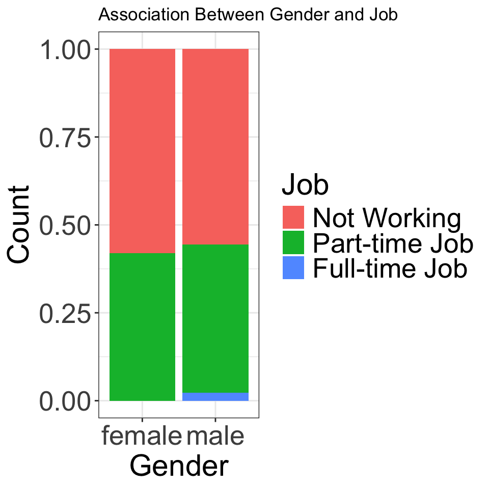
                    female       male
  Not Working   0.58035714 0.55555556
  Part-time Job 0.41964286 0.42222222
  Full-time Job 0.00000000 0.02222222
What does Independent Means?
Observed Proportions:
                    female       male
  Not Working   0.58035714 0.55555556
  Part-time Job 0.41964286 0.42222222
  Full-time Job 0.00000000 0.02222222
Observed Counts \(n_{ij}\):
                female male
  Not Working       65   25
  Part-time Job     47   19
  Full-time Job      0    1
Expected Counts under the Null (Independence):
| Job | female | male | Total |
|---|---|---|---|
| Not Working | |||
| Part-time Job | |||
| Full-time Job | |||
| Total |
Deviasion-based Test Statistic
- Expected Counts: \(e_{ij}=\frac{n_{i+}\times n_{+j}}{n}\)
- Deviation: \(n_{ij}-e_{ij}\)
- Test Statistic: \(\chi^2 = \sum_{all\ cells} \frac{(n_{ij}-e_{ij})^2}{e_{ij}}\)
- Assumption: Independence & Large \(n_{ij}\): -\(\chi^2\sim \text{ch-square}\left(df=(n_{row}-1)(n_{col}-1)\right)\)
Simulation-Based Test of Independence
- Test Statistic: \(\chi^2 = \sum_{all\ cells} \frac{(n_{ij}-e_{ij})^2}{e_{ij}}\)
- Assumption: Independence
- Shuffle one variable
- Calculate test statistics
- Repeat many times
- Create a histogram as Null Distributoin
CourseKata Ch. 11 (2)