CourseKata Chapter 11

Model Significance (1)

Mansour Abdoli, PhD

Overview / Goals

• Assumption \(\rightarrow\) Null Dist. \(\rightarrow\) Observation
• Theoretical Null Distribution
• Test of Significance: \(\beta_1\)
• Type I and Type II Errors

Assumption \(\rightarrow\) Null Dist. \(\rightarrow\) Observation

Sampling Variability

• Different samples → different statistics
• Statistics vary naturally

Key idea:

Variation is normal, not suspicious

Sampling Distribution

• Distribution of a statistic across many samples
• Built by:
  • Re-sampling OR
  • Mathematical theory

Null Distribution

Null Hypothesis (\(H_0\)):

• Assumption:
  • No effect
  • No difference
  • No relationship

• Null Distribution of \(b_1\):
  • Categorical Explanatory
    • Mean difference = 0
  • Quantitative Explanatory
    • Slope = 0

Null Distribution: Simulation

• Simulate no Association:
  • Shuffle Outcome
• Compute \(b_1\)
• Repeat many times
• Visualize (Histogram)
• Add the observed value

Theotetical Null Distribution

Null Distribution: Mathematical Model

• Assumption: Error Distribution \(\sim N(0, \sigma)\)

Categorical Explanatory

• Normal
• Mean of 0
• Same group variances
  

Quantitative Explanatory

• Normal
• Mean of 0
• Variance constant across \(X\)

• Null Distribution: \(\frac{b_1}{s_{b1}}\sim t(df=n-2)\)

• Sampling Distribution: \(\frac{b_1-\beta_1}{s_{b1}}\sim t(df=n-2)\)

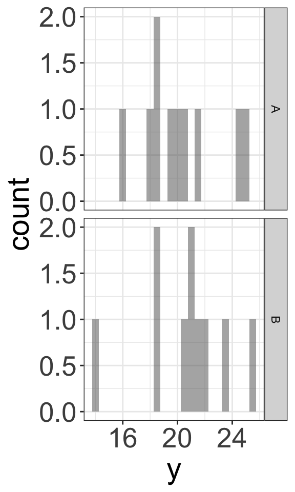
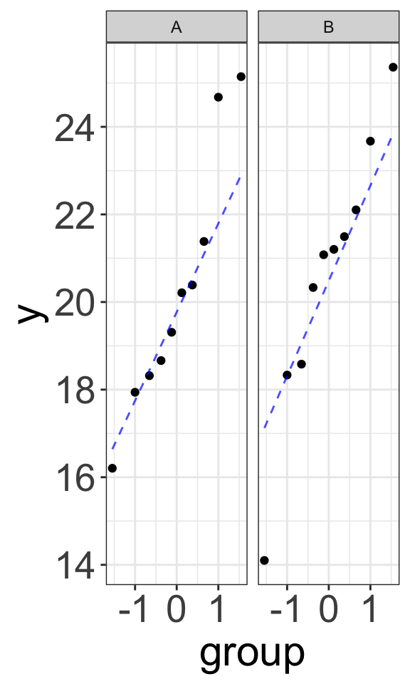
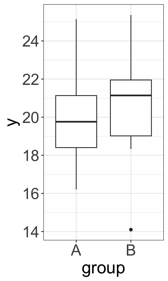
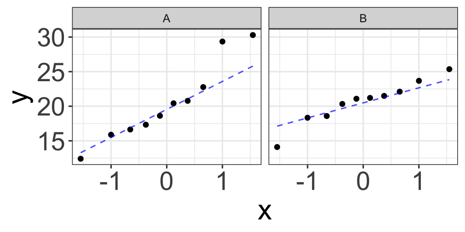
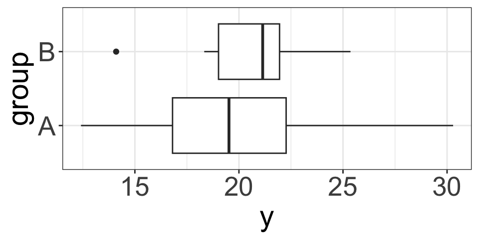
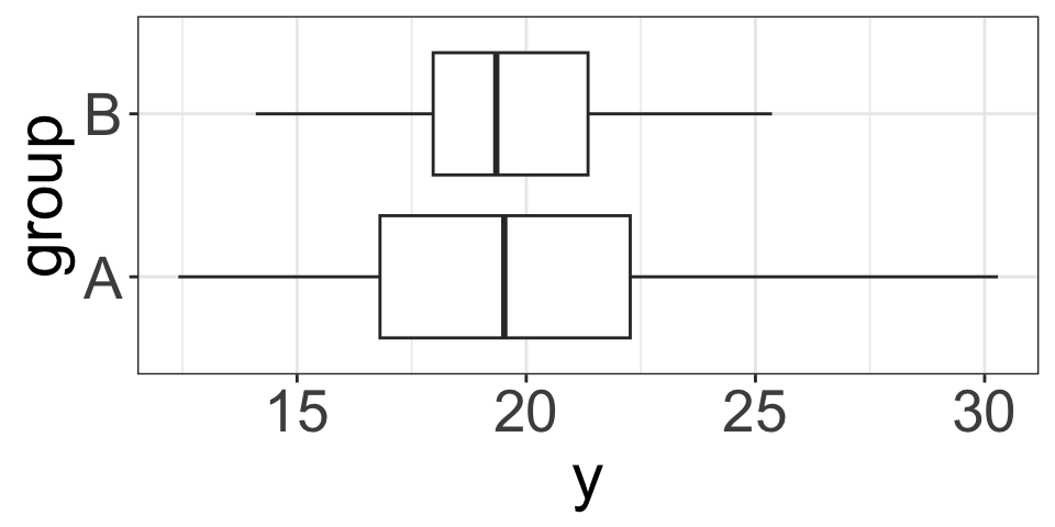
Example 1: Categorical Explanatory

\[Y_A\sim N(20, 3), \quad Y_B\sim N(20, 3), \quad n_1=n_2=10\]

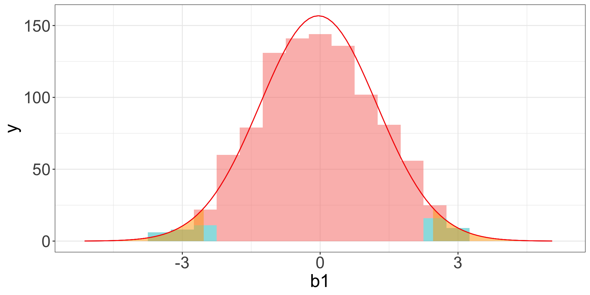
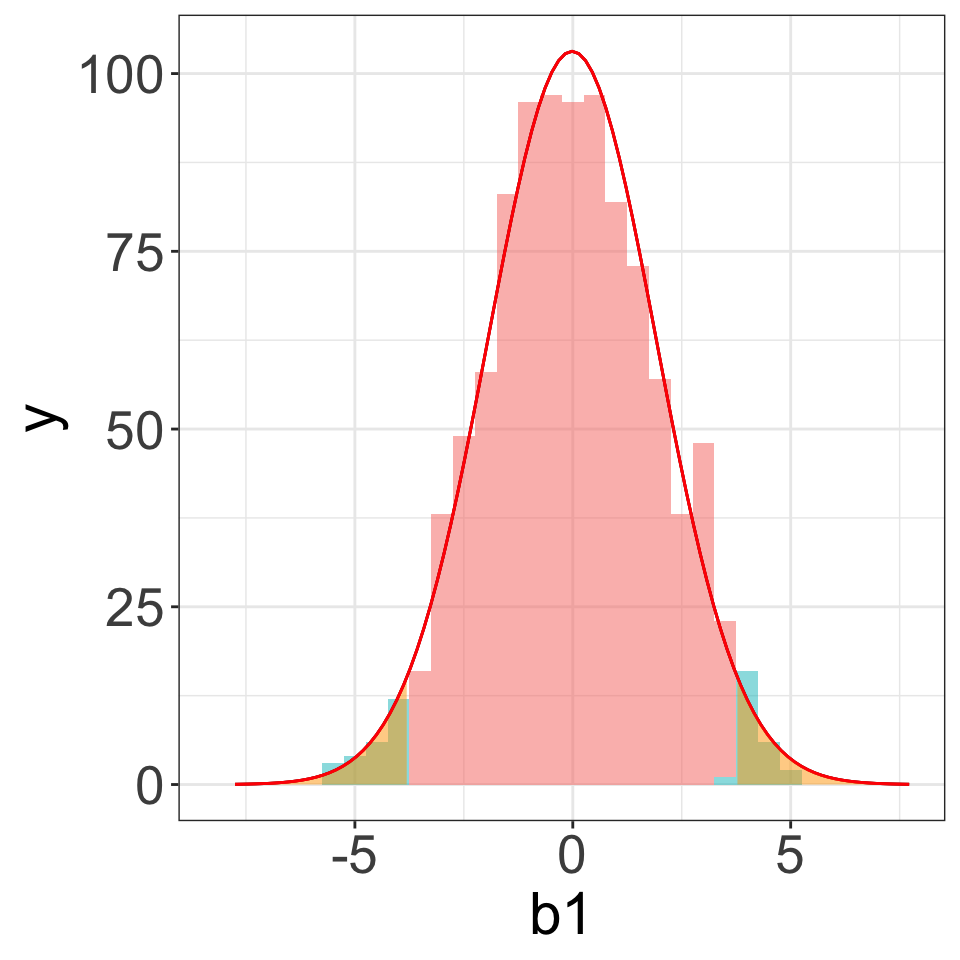
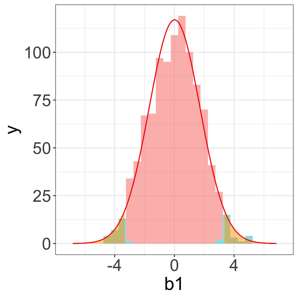
Example 1: Null Distributions

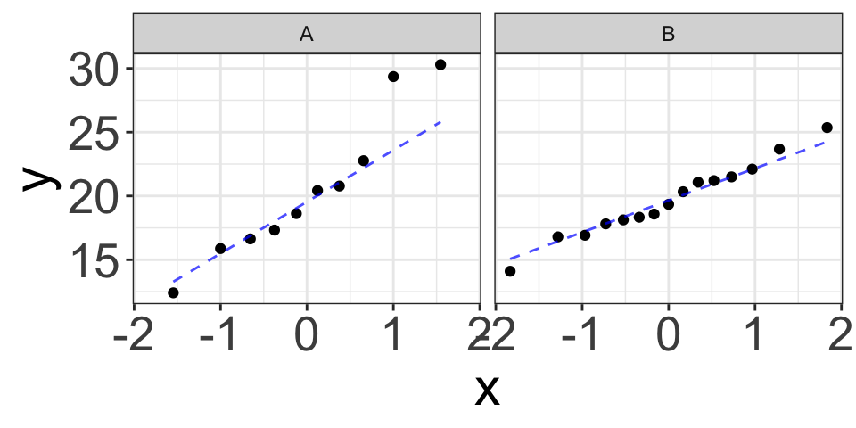
Example (2): Different Variance

\[Y_A\sim N(20, 6), \quad Y_B\sim N(20, 3), \quad n_1=n_2=10\]

Example (3): Unbalanced Data

\[Y_A\sim N(20, 6), \quad Y_B\sim N(20, 3), \quad n_1=10, n_2=15\]

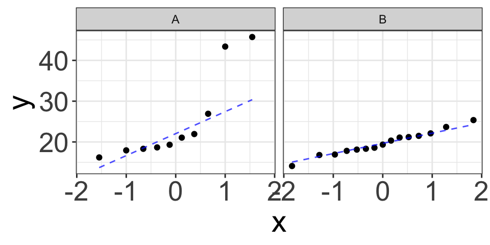
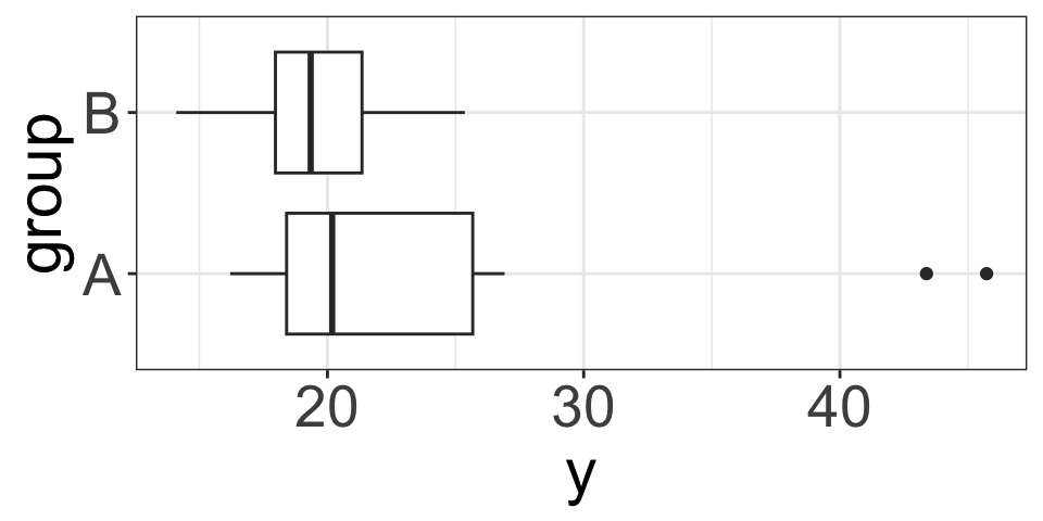
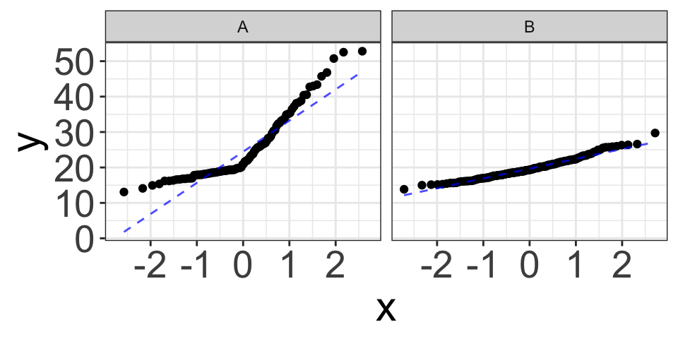
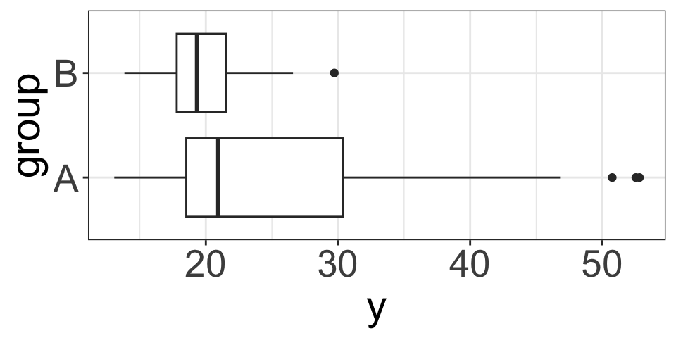
Example (4): Skewed Distribution

\[Y_A\sim N(20, 3), \quad Y_B\sim \text{skewed right}, \quad n_1=10, n_2=15\]

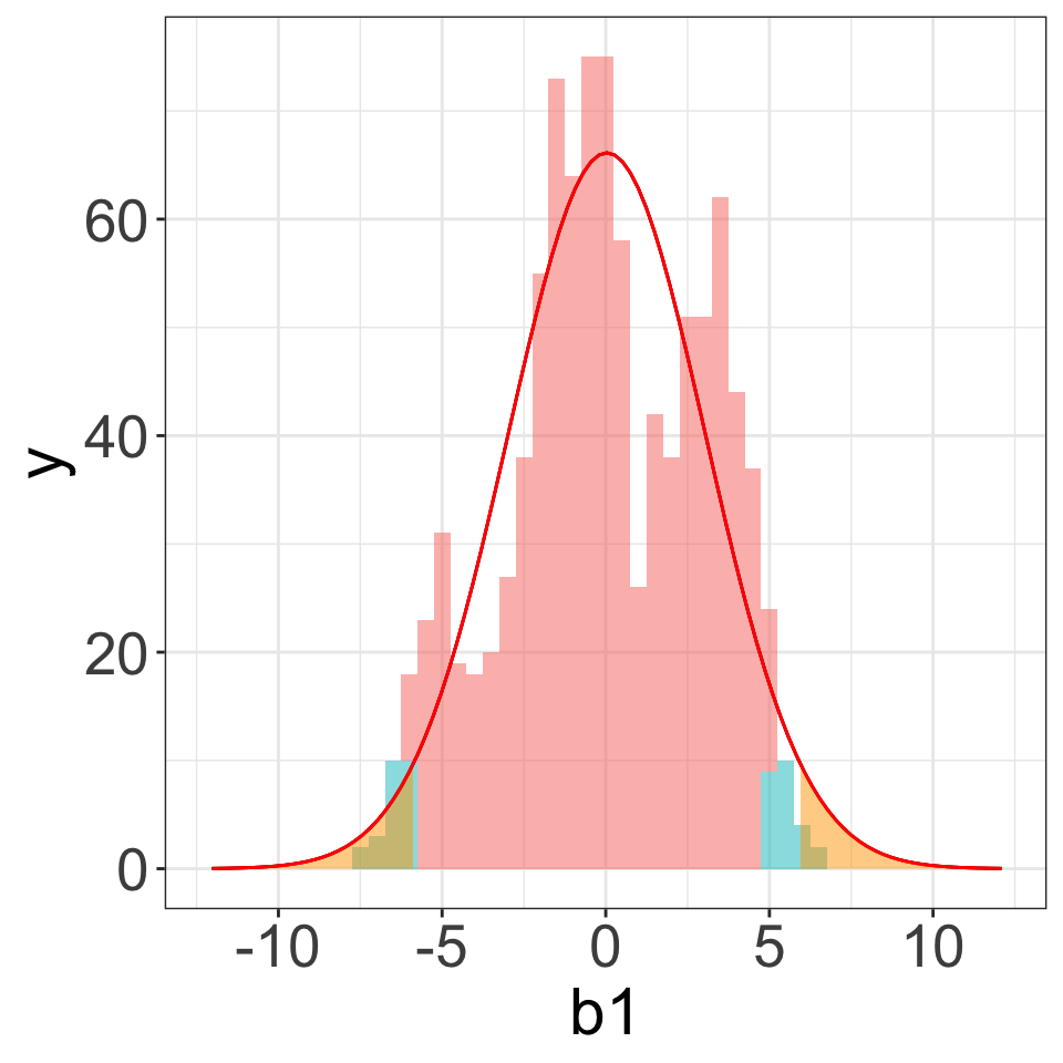
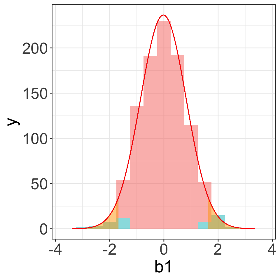
Example (5): Skewed & large \(n\)

\[Y_A\sim N(20, 3), \quad Y_B\sim \text{skewed right}, \quad n_1=100, n_2=150\]

Null Distribution Summary

For a binary numeriacl \(X\): \[Y=\beta_0+\beta_1 X + \varepsilon\] \[\frac{b_1-\beta_1}{s_{b_1}} \sim t(df=n-2)\]

• If assumptions met:
  • Error Distribution \(\sim N(0, \sigma)\)
  • \(n\) is large

• \(t(df)\):
  • a density centered at \(0\)
  • more spread than \(Z\)
  • as \(df (n)\to \infty, \quad t\xrightarrow{D} z\)

Test of Significance \(\beta_1\)

\(H_a\) & Unusual (Unexpected) Event

• Assumption & \(H_0 \to\) Null Distribution
• Alternative:
  • \(\beta_1>0\): Reject \(H_0\) if too far to the right.
  • \(\beta_1<0\): Reject \(H_0\) if too far to the left.
  • \(\beta_1\ne0\): Reject \(H_0\) if too far from the middle (expected).

Thumb~Gender Example

\[Thumb=\beta_0+\beta_1 Gender_{Male} + \varepsilon\] - \(H_0: \beta_1=0\) vs. \(H_a: \beta_1\ne 0\)

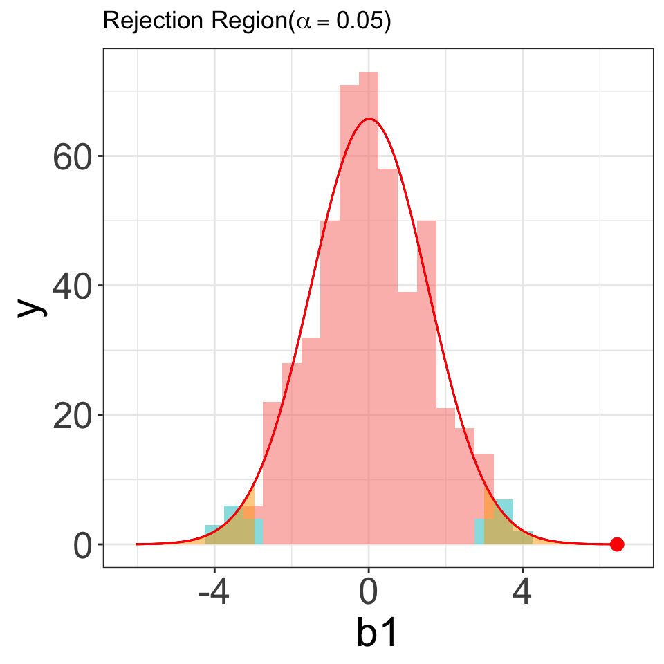
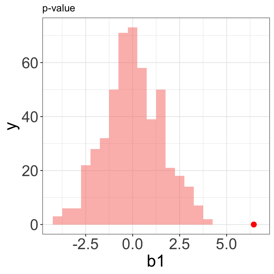
Probability of getting a result this extreme (or more) if the null is true

Decision

Reject \(H_0\), at \(\alpha\) significance level, if:

• Observed \(b_1\) is in Rejection Region

• \(p\)-value is less than \(\alpha\)

otherwise,

• Fail to reject \(H_0\)
• Both \(H_a\) and \(H_0\) are plausible.

Type I & II Errors

Type I Error

Rejecting a true null

• False Positive
• False Alarm

\[\begin{align*}\alpha &= P(\text{Rejecting } H_0|H_0) \\ \\ &=\frac{FP}{FP+TN}\end{align*}\]

Type II Error

Failing to reject a false null

• False Negative
• Missed Opportunity

\[\begin{align*}\beta &= P(\text{Not Rejecting } H_0|H_a) \\ \\ &=\frac{FN}{FN+TP}\end{align*}\]

Full Workflow

1. State the null & Alt. hypothesis
2. Find the null distribution of the test statistic
3. Compute the observed (test) statistic
4. Compute p-value or check against R.R.
5. Make a decision & write a conclusion
6. Check assumptions